Understanding Bayesian Updates with a Simple Gaussian Model

Bayesian inference is a framework for updating beliefs in light of new evidence. In this post we go through the formulas involved in estimating the mean of a gaussian dataset, along with code to do said process.

The Gaussian Distribution

A Gaussian (or normal) distribution is described by two parameters: the mean and standard deviation . Its probability density function (PDF) is given by:

In this example we generate synthetic data from a Gaussian distribution with a true mean and variance .

Using this data as our true data we then want to estimate by iteratively update our belief about using Bayesian inference.

We write this in python as:

import numpy as np
import matplotlib.pyplot as plt

# Define a Gaussian function
def gaussian(x, mean, std):
    return (1 / (np.sqrt(2 * np.pi) * std)) * np.exp(-0.5 * ((x - mean) / std) ** 2)

and we generate a synthetic dataset from this gaussian

# Generate data by sampling from a Gaussian
np.random.seed(42)
true_mean, true_std = 5, 2
n_samples = 1000
x_values = np.linspace(true_mean - 4 * true_std, true_mean + 4 * true_std, 1000)
distribution = gaussian(x_values, true_mean, true_std)
data = np.random.choice(x_values, size=n_samples, p=distribution / np.sum(distribution))

The variable data is now a list of observations from that distribution.

Bayesian Framework

Bayes' theorem is a fundamental theorem in probability theory that describes how to update the probability of a hypothesis based on new evidence. It is expressed as:

Where:

• is the posterior probability, the probability of the hypothesis given the data.
• is the likelihood, the probability of the data given the hypothesis.
• is the prior probability, the initial probability of the hypothesis.
• is the marginal likelihood or evidence, the total probability of the data.

We can rewrite this as:

Why is Used

The use of (proportional to) arises because Bayes' theorem includes a normalization constant, the evidence :

This ensures the posterior is a valid probability distribution. However, is independent of , so when calculating the posterior shape, we can write:

This simplification:

1. Avoids explicitly calculating , which can be computationally expensive.
2. Focuses on the relative contributions of the prior and likelihood.
3. Leaves normalization implicit, which is straightforward for Gaussian distributions.

Derivation of Posterior Updates

Prior and Likelihood

The prior and likelihood are both Gaussian distributions:

• Prior:

• Likelihood:

Posterior Distribution

Combining the prior and likelihood:

Expanding and grouping terms involving :

From this, we identify the posterior as a Gaussian distribution with updated parameters:

1. Posterior Variance:

2. Posterior Mean:

Iterative Updates with Multiple Observations

When observing multiple data points , the posterior is updated iteratively. After observations, the posterior parameters are:

• Variance:

• Mean:

This iterative process is implemented in the code, leading to convergence of the posterior mean and variance as more data is observed.

# Prior parameters
prior_mean, prior_var = 0, 10
# Likelihood parameters (assumed known)
likelihood_var = true_std**2

# Bayesian updates
posterior_mean, posterior_var = prior_mean, prior_var
means, vars = [], []

for i in range(n_samples):
    posterior_mean = (posterior_mean / posterior_var + data[i] / likelihood_var) / ( 1 / posterior_var + 1 / likelihood_var )
    posterior_var = 1 / (1 / posterior_var + 1 / likelihood_var)
    means.append(posterior_mean)
    vars.append(posterior_var)

posterior_std = np.sqrt(posterior_var)

print(f"True mean: {true_mean}")
print(f"Prior mean: {prior_mean} ± {np.sqrt(prior_var)}")
print(f"Posterior mean: {posterior_mean} ± {posterior_std}")

Results and Visualization

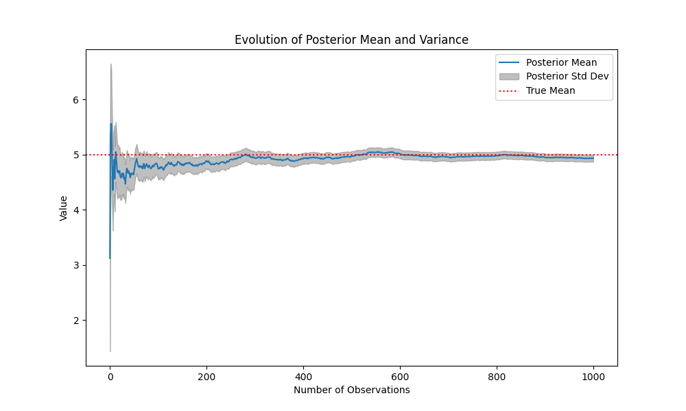
The Python implementation shows that as , the posterior parameters approach the true values:

Visualization:

The plot below illustrates the evolution of the posterior mean and variance over time:

• Posterior Mean: Converges to the true mean ().
• Posterior Variance: Shrinks, indicating increased confidence.

Full code: