Understanding Bayesian Updates with a Simple Gaussian Model

Bayesian inference is a framework for updating beliefs in light of new evidence. In this post we go through the formulas involved in estimating the mean of a gaussian dataset, along with code to do said process.

---

The Gaussian Distribution

A Gaussian (or normal) distribution is described by two parameters: the mean $\mu$ and standard deviation $\sigma$. Its probability density function (PDF) is given by:

$$f(x \mid \mu, \sigma^2) = \frac{1}{\sqrt{2 \pi \sigma^2}} \exp\left(-\frac{(x - \mu)^2}{2 \sigma^2}\right)$$

In this example we generate synthetic data from a Gaussian distribution with a true mean $\mu_{\text{true}} = 5$ and variance $\sigma_{\text{true}}^2 = 4$.

Using this data as our true data we then want to estimate $\mu$ by iteratively update our belief about $\mu$ using Bayesian inference.

We write this in python as:

import numpy as np
import matplotlib.pyplot as plt

# Define a Gaussian function
def gaussian(x, mean, std):
    return (1 / (np.sqrt(2 * np.pi) * std)) * np.exp(-0.5 * ((x - mean) / std) ** 2)

and we generate a synthetic dataset from this gaussian

# Generate data by sampling from a Gaussian
np.random.seed(42)
true_mean, true_std = 5, 2
n_samples = 1000
x_values = np.linspace(true_mean - 4 * true_std, true_mean + 4 * true_std, 1000)
distribution = gaussian(x_values, true_mean, true_std)
data = np.random.choice(x_values, size=n_samples, p=distribution / np.sum(distribution))

The variable data is now a list of observations from that distribution.

---

Bayesian Framework

Bayes' theorem is a fundamental theorem in probability theory that describes how to update the probability of a hypothesis based on new evidence. It is expressed as:

$$p(\mu \mid x) = \frac{p(x \mid \mu) \cdot p(\mu)}{p(x)}$$

Where:

• $p(\mu \mid x)$ is the posterior probability, the probability of the hypothesis given the data.
• $p(x \mid \mu)$ is the likelihood, the probability of the data given the hypothesis.
• $p(\mu)$ is the prior probability, the initial probability of the hypothesis.
• $p(x)$ is the marginal likelihood or evidence, the total probability of the data.

We can rewrite this as:

$$p(\mu \mid x) \propto p(x \mid \mu) \cdot p(\mu)$$

Why $\propto$ is Used

The use of $\propto$ (proportional to) arises because Bayes' theorem includes a normalization constant, the evidence $p(x)$:

$$p(x) = \int p(x \mid \mu) p(\mu) \, d\mu$$

This ensures the posterior is a valid probability distribution. However, $p(x)$ is independent of $\mu$, so when calculating the posterior shape, we can write:

$$p(\mu \mid x) \propto p(x \mid \mu) \cdot p(\mu)$$

This simplification:

1. Avoids explicitly calculating $p(x)$, which can be computationally expensive.
2. Focuses on the relative contributions of the prior and likelihood.
3. Leaves normalization implicit, which is straightforward for Gaussian distributions.

---

Derivation of Posterior Updates

Prior and Likelihood

The prior and likelihood are both Gaussian distributions:

• Prior:

$$p(\mu) = \frac{1}{\sqrt{2 \pi \sigma_{\text{prior}}^2}} \exp\left(-\frac{(\mu - \mu_{\text{prior}})^2}{2 \sigma_{\text{prior}}^2}\right)$$

• Likelihood:

$$p(x_i \mid \mu) = \frac{1}{\sqrt{2 \pi \sigma_{\text{true}}^2}} \exp\left(-\frac{(x_i - \mu)^2}{2 \sigma_{\text{true}}^2}\right)$$

Posterior Distribution

Combining the prior and likelihood:

$$p(\mu \mid x_i) \propto \exp\left(-\frac{(\mu - \mu_{\text{prior}})^2}{2 \sigma_{\text{prior}}^2}\right) \cdot \exp\left(-\frac{(x_i - \mu)^2}{2 \sigma_{\text{true}}^2}\right)$$

Expanding and grouping terms involving $\mu$:

$$p(\mu \mid x_i) \propto \exp\left(-\frac{1}{2} \left[ \mu^2 \left(\frac{1}{\sigma_{\text{prior}}^2} + \frac{1}{\sigma_{\text{true}}^2}\right) - 2 \mu \left(\frac{\mu_{\text{prior}}}{\sigma_{\text{prior}}^2} + \frac{x_i}{\sigma_{\text{true}}^2}\right) \right] \right)$$

From this, we identify the posterior as a Gaussian distribution with updated parameters:

1. Posterior Variance:

$$\sigma_{\text{posterior}}^2 = \frac{1}{\frac{1}{\sigma_{\text{prior}}^2} + \frac{1}{\sigma_{\text{true}}^2}}$$

2. Posterior Mean:

$$\mu_{\text{posterior}} = \sigma_{\text{posterior}}^2 \left(\frac{\mu_{\text{prior}}}{\sigma_{\text{prior}}^2} + \frac{x_i}{\sigma_{\text{true}}^2}\right)$$

---

Iterative Updates with Multiple Observations

When observing multiple data points $x_1, x_2, \dots, x_n$, the posterior is updated iteratively. After $n$ observations, the posterior parameters are:

• Variance:

$$\sigma_{\text{posterior}}^2 = \frac{1}{\frac{1}{\sigma_{\text{prior}}^2} + n \cdot \frac{1}{\sigma_{\text{true}}^2}}$$

• Mean:

$$\mu_{\text{posterior}} = \sigma_{\text{posterior}}^2 \left(\frac{\mu_{\text{prior}}}{\sigma_{\text{prior}}^2} + \frac{\sum_{i=1}^n x_i}{\sigma_{\text{true}}^2}\right)$$

This iterative process is implemented in the code, leading to convergence of the posterior mean and variance as more data is observed.

# Prior parameters
prior_mean, prior_var = 0, 10
# Likelihood parameters (assumed known)
likelihood_var = true_std**2

# Bayesian updates
posterior_mean, posterior_var = prior_mean, prior_var
means, vars = [], []

for i in range(n_samples):
    posterior_mean = (posterior_mean / posterior_var + data[i] / likelihood_var) / ( 1 / posterior_var + 1 / likelihood_var )
    posterior_var = 1 / (1 / posterior_var + 1 / likelihood_var)
    means.append(posterior_mean)
    vars.append(posterior_var)

posterior_std = np.sqrt(posterior_var)

print(f"True mean: {true_mean}")
print(f"Prior mean: {prior_mean} ± {np.sqrt(prior_var)}")
print(f"Posterior mean: {posterior_mean} ± {posterior_std}")

Results and Visualization

The Python implementation shows that as $n_{\text{samples}} = 1000$, the posterior parameters approach the true values:

$$\mu_{\text{posterior}} = 5.02, \quad \sigma_{\text{posterior}} = 0.06$$

Visualization:

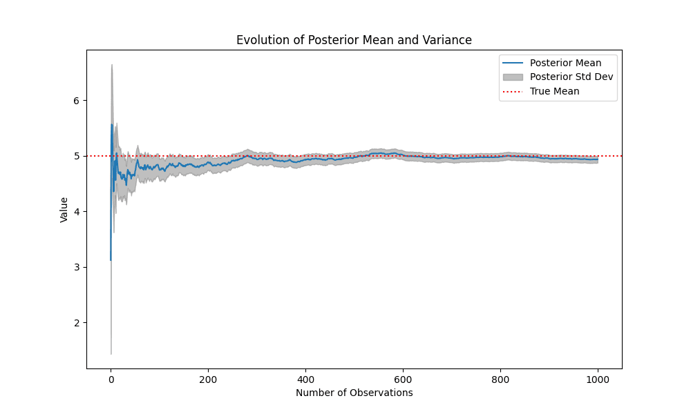
The plot below illustrates the evolution of the posterior mean and variance over time:

• Posterior Mean: Converges to the true mean ($\mu_{\text{true}} = 5$).
• Posterior Variance: Shrinks, indicating increased confidence.

---

Full code:

import numpy as np
import matplotlib.pyplot as plt

# Define a Gaussian function
def gaussian(x, mean, std):
    return (1 / (np.sqrt(2 * np.pi) * std)) * np.exp(-0.5 * ((x - mean) / std) ** 2)

# Generate data by sampling from a Gaussian
np.random.seed(42)
true_mean, true_std = 5, 2
n_samples = 1000
x_values = np.linspace(true_mean - 4 * true_std, true_mean + 4 * true_std, 1000)
distribution = gaussian(x_values, true_mean, true_std)
data = np.random.choice(x_values, size=n_samples, p=distribution / np.sum(distribution))

# Prior parameters
prior_mean, prior_var = 0, 10
# Likelihood parameters (assumed known)
likelihood_var = true_std**2

# Bayesian updates
posterior_mean, posterior_var = prior_mean, prior_var
means, vars = [], []

for i in range(n_samples):
    posterior_mean = (posterior_mean / posterior_var + data[i] / likelihood_var) / ( 1 / posterior_var + 1 / likelihood_var )
    posterior_var = 1 / (1 / posterior_var + 1 / likelihood_var)
    means.append(posterior_mean)
    vars.append(posterior_var)

posterior_std = np.sqrt(posterior_var)

# Results
print(f"True mean: {true_mean}")
print(f"Prior mean: {prior_mean} ± {np.sqrt(prior_var)}")
print(f"Posterior mean: {posterior_mean} ± {posterior_std}")

# Plot posterior evolution
plt.figure(figsize=(10, 6))
plt.plot(means, label="Posterior Mean")
plt.fill_between(
    range(n_samples),
    np.array(means) - np.sqrt(vars),
    np.array(means) + np.sqrt(vars),
    color="gray",
    alpha=0.5,
    label="Posterior Std Dev",
)
plt.axhline(true_mean, color="red", linestyle="dotted", label="True Mean")
plt.title("Evolution of Posterior Mean and Variance")
plt.xlabel("Number of Observations")
plt.ylabel("Value")
plt.legend()
plt.savefig("posterior_evolution_gaussian.png")
plt.show()